What made me think about this is the lack of a symbol which I wish to exist (please put me out of my misery if it already does). We don’t write $A\cup B = B$ or $A\cap B = A$ to say that $A$ is a subset of $B$. While logically correct, we invented a symbol for this common scenario. I would argue that stating whether two sets are disjoint occurs frequently enough to deserve a symbol. In both cases too! If $E\cap F = \emptyset$ then $\mu(E\cup F) = \mu(E) + \mu(F)$ and if $U_i \cap U_j \neq \emptyset$ then the transition map $\phi_{ij}$ should be smooth. I propose a symmetric symbol to denote whether two sets intersect non-trivially: the best I’ve found is $\between$ for ‘non-disjoint’ but I am open to suggestions!

“Go forth and generalise.”

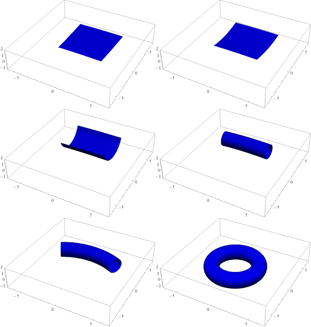
This post contains more information abouts donuts (tori herein), but to recap we build one by gluing together the opposite edges of a square:

Functions on the torus naturally arise as functions of two real variables which are periodic in both arguments. The specific functions on the torus that we’re interested in are the solutions to my favourite PDE:

Rather than working on the torus, denoted $\mathbb{T}$, it is easier to solve this equation on the square and then ask that the solution is periodic in both $x$ and $y$ with period $1$. Trusty separation of variables yields

which is an eigenfunction with eigenvalue

For $u_k(x,y)$ to be periodic we need

and by the definition of $u_k$, this means that

Renaming $k_x = m$ and $k_y = n$, we find that

The points $(m,n)\in\mathbb{Z}^2$ form a lattice. Is it a coincidence that the unit square we started out with tiles this lattice? More on that later…

Now we have the eigenfunctions of the Laplacian, the spectral theorem tells us that these form a basis for a friendly bunch of functions on the torus:

That is, every $f\in L^2(\mathbb{T})$ can be decomposed as

where

The advantage of the notation $\hat{f}$ over the usual $a_n$ or $c_n$ for a coefficient is to remind us that the coefficient depends directly on the function $f$. While $f$ is a function on $\mathbb{T}$, we’ll see later that $\hat{f}$ is a function on $\hat{\mathbb{T}}$.

Philosophically, the spectral theorem says that the Laplacian on a torus is diagonalisable, in the sense that

That’s the end of the example. I hope it’s clear that there is fecund ground for abstraction.

7. Ordinary

Got to start where it all started. You’re on a hike and you know what the elevation is at each point but you want to know how steep it is at each point i.e. what is the gradient? This is precisely the question ``What is the (ordinary) derivative of the elevation as a function of distance?”. Alternative to the usual slope interpretation, the derivative also measures the degree to which each point gets stretched or squashed when squeezing the domain into the co-domain.

6. Partial

I can look at how one location and compare how it changed over time: call this history. Alternatively I can look at a fixed point in time and compare different places: call this geography perhaps. What about something like the Roman empire which spread over time: I could follow the path of a Roman legion as it moves through space and time and measure something along its path: this would be called a directional derivative. As I said in the post on partial differential equations, most things depend on more than one thing and so it’s important we know how something responds to changes in the various things it depends on.

5. Material

Imagine a bear sitting on the bank of a river with a fishing rod. It looks at the river and wonders how fast it’s flowing at each point. It could take a snapshot in time and look at how the flow of the river changed from point to point. It could also look at a point in the flow and see how the flow changes over time, say by attaching a detector to the river bed. However this is only one perspective (called the Eulerian one). If I were a fish being carried along in the flow, hoping to avoid the bear’s fishing rod, (whaling, fishing, crabbing are the only examples I can think of where turning an animal’s name into a verb means to hunt that animal) I would experience speeding up, slowing down and changing direction. This is a more natural way to phrase the laws of fluid mechanics. A point that is carried along in the flow is affected by its neighbouring points which are carried along in the same flow. This idea is encapsulated by the material derivative. I talk about this in more depth in my Navier-Stokes post.

4. Weak

Suppose I want to loosen the sense of what it means for a function to have a derivatve. I can only differentiate some functions but I can integrate way more functions. Therefore it makes sense to ask for functions that satisfy conditions in integrals: integrals are blind to finite sets of points (and even sets of measure zero) and so is more lenient to functions with pesky discontinuities in their derivative like the absolute value $f(x) =\mid x\mid$. The way we phrase this is that a function is weakly differentiable if we can do integration by parts on it. Specifically, $u$ has weak derivative $v$ if for all smooth functions $\phi$,

A small problem: by broadening the class of possible solutions to an equation, we’ve exchanged uniqueness for existence. Two different functions can satisfy the above condition which disagree on a set of measure zero. The boundary of a domain is a set of measure zero so what does it even mean for a weak solution to satisfy a boundary condition?

3. Radon - Nikodym

I want to assign sizes to parts of a material in a consistent way. Two possible ways for me to do this are by measuring the volume or the mass of a chunk. Volume might seem like the natural choice but mass is just as good and they are related by the fact that if I know the density of the material (a positive function) $\rho$ then the mass of a subset, denoted $M(E)$, is related to the volume of that subset, denoted $V(E)$, by

So in a sense we can build new measures (ways of assigning size to sets) out of old ones using a density function. The Radon-Nikodym theorem goes the other way and states that if I have two measures $\mu$ and $\nu$ with the property that $\nu(E)$ is $0$ whenever $\mu(E)$ is $0$ (specifically $\nu$ is absolutely continuous with respect to $mu$ which is written $\nu \ll \mu$) then there is a non-negative density function $f$ so that

and the density is called the Radon-Nikodym derivative and denoted $f = \frac{d\mu}{d\nu}$.

2. Exterior

The ordinary derivative, the gradient of a function and the curl of a vector field are all examples of the exterior derivative. This is a huge generalisation of familiar derivatives and some of our favourite facts from calculus are just examples of powerful theorems in differential geometry. If the exterior derivative is denoted $d$ then the fundamental theorem of calculus, Stokes theorem and the divergence theorem are all just examples of the fact

Furthermore, facts like ‘the curl of a gradient vanishes’ and ‘the divergence of a curl is zero’ are special cases of the succinct fact

(as an operator).

1. Covariant

“A tensor is something that transforms like a tensor” is a horrible description but I don’t have much better. General relativity seeks descriptions of a physical system which are independent of the observer making the description. Changes in perspective between observers manifests as coordinate transformations so we would like to keep track of how quantities change under coordinate transformations so that we’re all measuring the same things. The gradient of a function is a tensor because if I scale my coordinate system in some way then by the chain rule the gradient will scale by some overall factor. But if I take the gradient of a tensor rather than a function and I change coordinates then the tensor will pick up a factor but the gradient is now acting on a product so I get a sum of terms. This is not how a tensor transforms and so our typical partial derivatives can’t define a tensor. Thankfully we can define a new tensor by subtracting off that extra term that comes out of the product rule to construct something that does transform like a tensor: the covariant derivative. And this is what allows us to take derivatives in relativity and thus express some pretty important laws.

We begin with a fact so fundamental it is called the fundamental theorem of arithmetic:

(1) Every number can be written, in a unique way, as a product of prime numbers.

This is taught as factor trees e.g. $48 = 3 \times 16= 3\times 2^4$, $49 = 7^2$, $50 = 2\times 5^2$. Now for another fact

(2) If two numbers can both be written as a SoS then their product can also be written as a sum of squares

for examaple,: $5 = 2^2 + 1^2$, $13 = 3^2 + 2^2$, $5\times 13 = 65 = 8^2 + 1^2 = 7^2 + 4^2$. Notice that I haven’t actually told you how we find the sum of squares of $65$ from the sums of squares of $5$ and $13$, only that it’s possible. A formula exists (Brahamgupta’s) but I won’t include it lest this post stops being kid friendly. The first two facts mean that we can work out which prime numbers are SoS because if all a number’s prime factors are SoS then the number must be too.

(3) Every prime number (other than $2$) has remainder $1$ or $3$ when divided by $4$

e.g. $3,7,11,19$ are all remainder $3$ and $5,13,17$ are all remainder $1$. If a number had remainder $0$ it’d be a multiple of $4$ so wouldn’t be prime and if it had remainder $2$ then it’d be even. Notice that just because a number has remainder $1$ that doesn’t make it prime e.g. $9 = 4\times 2 + 1 = 3^2$. From now on ‘remainder $1$’ and ‘remainder $3$’ always mean ‘when divided by $4$’.

(4a) A prime number that is remainder $1$ can be written as a SoS

(4b) A prime number that is remainder $3$ cannot be written as a SoS

(4c) $2$ is the only prime number which is remainder $2$ and can be written as $2 = 1^2 + 1^2$.

I have to mention that it is easy to prove the contrapositive of (4b) but the proof of (4a) requires Legendre symbols. Using the first four facts we can now partially answer whether a number can be written as a SoS. e.g. $325 = 5\times 65 = 5\times 5\times 13$ and $5$ and $13$ are both prime numbers which are remainder $1$ so by fact (4a) they can be written as a SoS and then by fact (2) $325$ can be too because it is a product of numbers that can and indeed $325 = 18^2 + 1^2 = 15^2 + 10^2$. On the other hand e.g. $39 = 3\times 13$ and can’t be written as a sum of squares. However $45 = 3^2 \times 5$ which can be written as a sum of squares ($45 = 6^2 + 3^2$) even though it has a prime factor which is remainder $3$ so our current method can tell us which numbers can be written as SoS but it is not yet able to tell us whether a number cannot be written as a SoS.

(5) If a number can be written as a SoS then that number multiplied by a square number can still be written as a sum of squares.

e.g. $5 = 2^2 + 1^2$ and $45 = 3^2 \times 5 = 3^2(2^2 + 1^2) = 3^2\times 2^2 + 3^2 \times 1^2= (3\times 2)^2 + (3\times 1)^2 = 6^2 + 3^2$.

A number which is a product of prime numbers which are remainder $1$ can be written as as sum of squares and multiplying by a square number or a power of $2$ doesn’t change whether a number can be written as a sum of squares. Now we have all the pieces.

(6) A number can be written as a SoS if and only if when decomposed into prime factors, all the primes which are remainder $3$ multiply together to make a square number.

Finally, some examples

1. $234 = 2\times 13 \times 3^2 = (1^2 +1^2)\times (3^2 + 2^2) \times 3^2 = (5^2 + 1^2) \times 3^2 = 15^2 + 3^2$ so $13$ is a remainder $1$ prime and multiplying by a power of $2$ and a square number doesn’t change the fact that it can be written as a SoS.
2. $40 = 8\times 5 = 2^2 (2 \times 5) = 2^2(1^2+1^2)(2^2 + 1) = 2^2(3^2 + 1^2) = 6^2 + 2^2$
3. $25 = 5 \times 5 = (2^2+ 1^2)(2^2 +1^2) = 3^2 + 4^2$
4. $98,000 = 98 \times 10^3 = 2\times 7^2 \times 2^3 \times 5^3 = 5 \times (7\times4\times 25)^2 = 5\times 700^2 = (2^2 + 1^2)\times 700^2 = 1400^2 + 700^2$

Differentiation as a matrix

One of the first things we learn about differentiation is that it is linear, which is something we end up using reflexively. If I ask you to differentiate $ex^2 + \pi x + \gamma$ then it doesn’t matter that this is a quadratic I’m sure you’ve never seen before: it’s a linear combination of functions you do know how to differentiate and so it poses no problem. More formally, differention is a linear map from functions with one continuous derivative to continuous functions, i.e. $D:C^1(\mathbb{R})\rightarrow C(\mathbb{R})$. And we know that, after we’ve picked a basis, linear maps on vector spaces can be represented by matrices. Unfortunately $C^1(\mathbb{R})$ doesn’t have a nice basis for me to work with so I’m going to restrict my attention to the vector spaces of polynomials. The monomials (shouldn’t it be mononomials?) form a nice basis for the polynomials and we know that the columns of a matrix in a basis are just the images of the basis elements under that map. Because $D:1\mapsto 0$, $D:x\mapsto 1$, $D:x^2\mapsto 2x$ i.e. derivatives reduce the order of a monomial by one, the matrix has non-zero entries only on the superdiagonal:

By writing differentiation as a matrix we can study ODEs using techniques from linear algebra. When I first saw this in my first term of undergrad it blew my mind: calculus is curvy and linear algebra is straight and never the twain shall meet. But little did I know this was the beginning of a very happy marriage with a healthy baby called function spaces.

PDEs as bilinear forms

Fast-forward 3 years and I’ve studied a bit of PDEs and some Hilbert spaces. Taking my Poisson’s equation on a domain $\Omega$

if we multiply by any test function (compactly supported and infinitely differentiable) $\phi$ and integrate over $\Omega$ we can use integration by parts to move a derivative from $u$ to $\phi$ to find

Any eigenfunction satisfies this equation but we’ve now formulated it in a way that only asks $u$ to have one derivative. Thus we can loosen the sense in which we ask a function to be an solution: a weak solution of Poisson’s equation is one that satisfies the above equation for all $\phi\in C^\infty_C(\Omega)$. As with any PDE we would like to know about the existence and uniqueness of a solution. If we define the bilinear form associated to the Laplacian by

then the weak form of Poisson’s equation is asking for a $u$ such that

for all $v$, where $(\cdot,\cdot)$ denotes the $L^2$ inner product. Fortunately this is the content of the Lax-Milgram theorem, which guarantees existence and uniqueness of a $u$ given some constraints (boundedness and coercivity) on $B$. Of course I haven’t addressed which Hilbert space we’re working in for this to make sense (it’s a Sobolev space) but it’s clear that the theory of PDEs cannot stand alone without the support of vector space methods.

Derivatives are linear maps

I am not just saying that differentiation is a linear map: I am also saying the output, a derivative, is itself a linear map. For functions of one variable this is subtle. The derivative evaluated at a point gives the ‘slope’ of the curve at that point which is just a number. Of course in one dimension a linear map is specified by a single number so at this resolution we cannot distinguish. However when we move up to functions of more variables the derivative is the gradient $\nabla f = (\partial_1 f, \partial_2 f,\cdots,\partial_n f)$. If I evaluate this at point $\mathbf{x_0}$ then $\nabla f(\mathbf{x_0})$ is a fixed vector and defines a linear map by acting on a unit vector $\mathbf{n}$ via $\nabla f(\mathbf{x_0}) \cdot \mathbf{n}$ to tell us the rate of change of the function $f$ in the direction $\mathbf{n}$ at the point $\mathbf{x_0}$. Thus when evaluated at the point $\mathbf{x_0}$, $\nabla f(\mathbf{x_0})$ belongs to the dual space of $\mathbb{R}^n$. Differential geometry generalises the hell out of this but we’ll only give the definition that a $0$-form is just a smooth function and a $1$-form is a smooth map from an open set in a vector space (like the domain of our function $f$) to the dual space of that vector space. Given a basis of $\mathbb{R}^n$ like $e_1,e_2,\cdots,e_n$ there is a dual basis $e_1^* ,\cdots,e_n^* $ such that $e_i^* (e_j) = \delta_{ij}$ and we can write the derivative in this basis as

Paul Erdős, the most published mathematician of all time, though agnostic, referred to god as the Supreme Fascist and believed that he held a book of the perfect proof of every theorem in maths. He would exclaim “This one’s from The Book” when he saw a particularly elegant proof and the first of our proofs is undoubtedly one of these.

Suppose, for contradiction, that there are a finite number of primes. I’m going to consider the resulting number when I multiply all these finitely many primes together and add 1. This new number is not divisible by any of the primes. Indeed it leaves remainder 1 when divided by any prime, and so its only factors can be itself and 1, meaning I’ve generated a new prime. This contradicts the assumption that I could collect the finitely many primes. This proof is certainly from the book. But why stop there?

Goldilocks stumbled across that proof and decided it didn’t require enough machinery. She tried the next one out for size.

The Riemann zeta function is a bit of a holy grail in mathematics, its zeros having a million dollar bounty, but we can still handle it with elementary methods. The harmonic series (the subject of the sequel to the ant on the rope post) and the Basel problem are both examples of the Riemann zeta function:

We can generalise the exponent in the sum and define the so-called Riemann zeta function:

There is an intimate link between this sum and the prime numbers. Consider the following method, analogous to the sieve of Eratosthenes. Multiply the sum by $1/2^s$ so that every denominator picks up a factor of $2$:

If we subtract this from the original sum then we remove all the even terms so we find

Now we do the same multiplying by $1/3^s$:

And subtracting this removes all denominators with a factor of 3:

If we proceed with each prime then we remove every term in the sum except for 1

Dividing and using some compact notation gives the prime product formula for the Riemann zeta function:

This is in fact more detail than we needed but I wanted to keep $s$ general to show why we might care about the Riemann Zeta function. If we evaluate at $s=1$ then we get the harmonic series which blows up to infinity:

But if the right hand side were a finite product it would have a finite value which would be a contradiction, hence there are infinitely many primes.

Goldilocks felt this was overkill. She tried out the following proof, hoping to strike a nice middle ground. We can define a topology on the integers whereby the open sets are generated by arithmetic sequences:

We can show that in this topology all open sets are closed. If I remove an arithmetic sequence from the integers then I can split what remains into shifted arithmetic sequences with the same common difference:

Taking complements shows that all open sets are also closed. Now we consider the following equation which says that every integer has a prime factor except for 1 and -1:

If there were finitely many primes then the left-hand side would be closed as a finite union of closed sets, however that would mean ${1,-1}$ was an open set which it is not. Therefore there cannot be finitely many primes. Goldilocks thought this proof was just right.

To begin with, what actually is a spectrum? The word comes from the Latin specere meaning to view and so a spectrum is an image. Originally this was the term given to the band of light which has been split by a prism; the term was later extended beyond visible wavelengths to the entire electromagnetic spectrum and later loosened to just mean the entire range, such as the autistic spectrum.

When heated, each element emits specific wavelengths of light. These wavelengths of light are like a fingerprint, uniquely identifying the element (the identification is called spectroscopy). In fact this is how Helium got its name: an unknown spectral line was detected during an eclipse.

Let’s look at the spectrum of the Hydrogen. Hydrogen is a fairly simple quantum system, consisting of an electron orbiting a proton. It was Max Planck who realised that the electron can only orbit at certain distances from the nucleus and so requires ‘packets’ energy (or quanta) to move between levels. Thus when an electron drops down a level it emits a photon with a particular amount of energy and the amount of energy is related (inversely proportionally) to the wavelength of emitted light. The gaps between energy levels are different, explaining why there are different wavelengths in the spectrum.

For a better idea of why the electron can only orbit at certain distances from the orbit, we need to remember that an electron is both a particle and a wave. This wave is wrapped around the nucleus so must oscillate some whole number of times in order to match up. The further away the electron sits, the more oscillations can be fit around its orbit. This can also be thought of as the quantisation of angular momentum.

But I don’t study electrons, I study functional analysis so how are quantum systems related to analysis? In quantum mechanics we treat quantities like energy and momentum no longer as numbers but as operators (in reality this involves putting a hat on a quantity like the position $x$ to make it an operator $\hat{x}$). Specifically, observable quantities are represented by Hermitian, linear operators. For the sake of simplicity we can think of them as matrices and when we make a measurement, for example an energy measurement, we can only get an eigenvalue of the matrix which corresponds to the energy of the system. Now it becomes very important to understand the eigenvalues of operators and especially those which correspond to physical observables.

Returning to the example of light, we can write down concretely the operator corresponding to the energy of an electron orbiting a proton and we can find its eigenvalues. Not every value can be an eigenvalue: the spectral theorem states that the spectrum of a (self-adjoint, compact, linear) operator is discrete so contains a countable sequence of values and QM tells us that the differences between them are the energies of photons which are emitted when electrons move between energy levels.

While the name only refers to light, the applications of spectral theory are much broader. Often we can cast a partial differential equation, for example the time independent Schrodinger equation, the heat equation or the wave equation, as an eigenvalue problem and employ the tools of spectral theory to synthesise the problem.

Aside 1: while writing this I realised that not a single common quantity has an operator which begins with the same letter: energy gets H, position gets x, momentum gets p and angular momentum gets L.

Aside 2, for those inclined: spectral theory in finite dimensional vector spaces is a little dull. We form the characteristic polynomial for a matrix and by the fundamental theorem of algebra we are guaranteed n roots, counted with multiplicity. Things get far more interesting in the infinite dimensional case: lets examine the equation $(T- \lambda I)x = 0$ a little more closely. In finite dimensions we have a theorem about when this equation has a non-trivial solution: precisely when the map $T-\lambda I$ has determinant 0. But in infinite dimensions we have no such criteria as to when the map $T-\lambda I$ is not invertible: not being bijective entails failing to be injective or surjective. In finite dimensions these concepts are equivalent but no longer. As a result we define firstly the resolvent set:

and the complement of the resolvent set in the complex numbers is the spectrum. Specifically if the map $T-\lambda I$ is not injective then there is a non-zero $x$ such that $(T-\lambda I)x = 0$, precisely the statement that $x$ is an eigenvector. The spectrum contains eigenvalues but also other points which only appear in infinite dimensional spaces, called the residual and continuous spectra. Further reading is left for the curious reader.

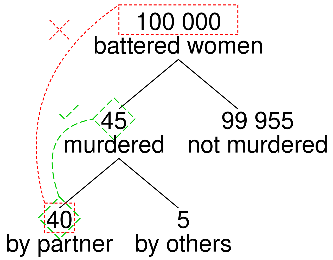
In 1995 O.J. Simpson was acquitted of the murder of his ex-wife Nicole Brown and her friend Ronald Goldman. During the trial, it was accepted that Simpson had been violent towards Brown when they were married. The defence argued that only 1 in 2500 women who experience spousal abuse are murdered by their partner and so the probability Simpson murdered Brown was low. However, this is a gross misuse of conditional probability.

For concreteness, imagine 100,000 women who are victims of domestic violence. Before Brown was killed, it is true that the probability she would be killed by Simpson was 40/100,000 = 1/2500. However the Bayesian framework tells us that once we learn of her murder, we must update our probability: no longer is she one of 100,000 victims of domestic abuse but she is now one of the 45 women who are victims of domestic abuse and have been murdered. Of those 45 women, 40 are killed by their partner and so the correct probability is 40/45, not the proposed 40/100,000.

Sally Clark

Sally Clark, a British solicitor, was accused in 1998 of murdering both her children at 11 weeks and 8 weeks old respectively. The prosecution asserted that the probability of 2 children suffering from Sudden Infant Death Syndrome (SIDS) was 1 in 73 million, a figure they found by taking the underlying population rate and squaring it. The tacit assumption here was that the events were independent. As all A level students know, and many of us intuitively understand, if two events are independent then the probability of them both occurring is the product of their individual probabilities. In this case this was a baseless assumption given there is a genetic predisposition to SIDS.

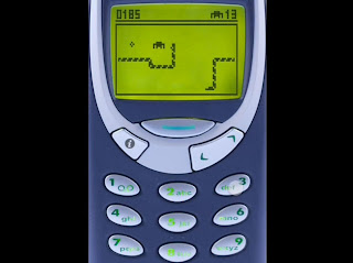
Clark was convicted but the ruling was later overturned when it was revealed that the prosecution forensic pathologist had withheld exculpatory evidence. The case caused hundreds of similar cases to be re-examined and as a result two other women had their convictions overturned.

In some sense we can think about one edge being the same edge as the opposite edge. In 2 dimensions the only way to visualise this is with the snake crossing one edge to come back out the other side but thankfully we have access to 3 dimensions. I can glue one pair of edges together to form a cylinder and then glue the circular ends of the cylinder together to form a doughnut shape, called a torus.

And so this game which allows you to play snake on a torus and claims to be a fun spin off is in fact identical to the original game.

Importantly, the square was 2 dimensional and so is the torus. When I talk about the torus I really mean the surface of the hollow doughnut, not the inside. Think of an inflatable ring for swimming rather than a bagel.

Having seen that a torus is a rectangle with its edges identified you can hopefully appreciate that its relatively easy to find the frequencies that can emanate from a torus-shaped drum - just find the frequencies that can exist on a rectangular drum and impose periodic boundary conditions.

Topology is an area of maths often referred to as rubber-sheet geometry. In geometry we can define quadrilaterals as a class of shapes without caring about their area, side lengths, or angles: only that they have 4 edges. Topology further relaxes the constraints required for two shapes to belong to the same class. In topology we say that two shapes are the same (homeomorphic) if they can be continuously defomed into one another, without any cutting or gluing. For an amazing introduction to topology I direct you to Vsauce’s ‘How many holes does a human have’.

Quite quickly it becomes clear that most shapes we distinguish geometrically (cubes, stellated polyhedra, cows) are all topologically homemorphic to the sphere. Topology is the search for quantities which remain unchanged by continuous deformations (topological invariants). We can use these invariants to determine whether two shapes are homeomorphic or not without finding an explicit transformation between them or, even more difficult, showing that no such transformation exists.

It is a powerful result (the Classification theorem) that every (orientable, compact, connected, boundary-less) surface can be classified simply by the number of holes it has (its genus) and so the torus is the ‘simplest’ shape which isn’t homeomorphic to a sphere - it has just 1 hole. After a donut we have a pair of handcuffs and a fidget spinner.

One fundamental difference between the sphere and the torus is that the latter is not simply connected. If I take a loop on the surface of a sphere, I can shrink it (staying on the surface) to a point on the sphere. Pretty quickly I can image a loop on the surface of a torus which can’t be shrunk to a point on the surface: it “gets caught on the hole”.

Our construction of the torus involving gluing the edges of a square together can be phrased a little more algebraically. We can define an equivalence relation on $\mathbb{R}$ by identify points with the same decimal part, or that differ by an integer. Then every equivalence class has a representative in the interval $[0,1)$, where $1$ and $0$ are identified, so the quotient of $\mathbb{R}$ by $\mathbb{Z}$ is isomorphic to the circle. What about points in the Euclidean plane? Then I can define the same equivalence relation: that a pair of points are equivalent if they differ additively by an element of $\mathbb{Z}^2$ so that all my equivalence classes have a representative in the unit square where I now identify the edges, forming a torus as I described before. In this case I would write something like $\mathbb{T}^2 \cong \mathbb{R}^2/\mathbb{Z}^2 \cong S^1 \times S^1$: a point on the torus can be defined by two angles. This gives us a way to easily define higher dimensional analogues of the torus, as well as classifying any torus as $\mathbb{R}^2$ modulo some lattice.

There are quantities which depend on one thing: the easiest example is a population depending on time. A differential equation is a relationship between something’s growth rate and its size. In a population that has some reproduction rate, the sentence ‘the larger the population, the faster it grows’ encodes a differential equation. Another example is radioactive decay: if I have a block of uranium then after some amount of time, half of it will have decayed. Then after another half-life, another half will decay. This is the same as the population example, but now ‘the larger the size, the faster it decays’. These are the two simplest differential equations we can describe, both written as $y’ = ky$ with $k$ positive in the first case and negative in the second.

There are myriad other examples where we measure something depending on one thing, usually time. For example, a pendulum swings and the angle it makes with the vertical depends on time. Or there’s a rocket flying away from Earth which burns fuel to propel itself and we can talk about its acceleration changing as its mass decreases. Another example is if I punch a hole in the bottom of a vat and in I pour in squash at a fixed rate at the top: what is the concentration of the squash as time evolves?

In all of these examples the quantity we’re measuring (population, distance, concentration, angle, mass) depends on only one number (in every case, time). For this reason they are all examples of ordinary differential equations. But these are all quite simple systems and in general things depend on more than one thing. A relationship between a quantity and it’s dependence on multiple different things is called a partial differential equation. Not because it’s any easier to solve, that’s some unfortunate nomenclature, but because the derivatives are only partial, i.e., they only take into account change with respect to one variable. My best example of this is the height of a string or the temperature along a rod. Both of these numbers depend on both my position along the rod/string and the time that I’m there.

The beauty of PDEs is the breadth of situations they encapsulate. The physical scale is astounding: Schrödinger’s equation describes the time evolution of quantum states of subatomic particles. Einstein’s equations describe the relationship between energy, mass and the curvature of spacetime on a cosmological scale. The Navier-Stokes equations (which I’ve now written 2 posts on) can be adapted both for the swimming of microorganisms or the flow of plasma comprising stars. PDEs range from the concrete, such as the Black-Scholes equation which describes the price evolution of financial derivatives, to the abstract, such as the Euler-Lagrange equations which state that every physical path is a minimizer of some action. There is a unifying aspect too: the same equation describes the diffusion of a pollutant in a body of water and the diffusion of heat throughout a body. The same equation describes incompressible, irrotational fluid flow, electromagnetic field configurations and the stable configurations of an elastic membrane. Heat and wave evolutions are unified through the Helmholtz equation.

But it is not the applications that interest me: mathematically, these are interesting objects to study in their own right. They are devilishly difficult to solve in generality (see the Navier-Stokes post) but we can still say so much about the solutions without knowing what they are.